Syria 2024/2025 Drought Season
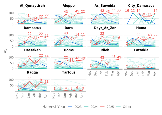
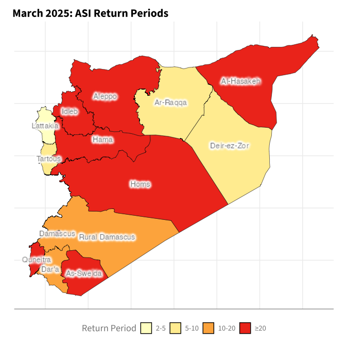
This section analyzes the evolution and spatial distribution of the Agricultural Stress Index (ASI) across Syrian governorates during the critical 2024/2025 winter cropping season (November 2024 to April 2025), a period highlighted in FAO’s drought alert as the most severe in 36 years.
We use ASI data obtained through the cumulus R package via FAO GIEWS, filtered by province and dekad to explore stress trends across crop-growing areas.
Code
<- function (x, direction = c ("1" , "-1" ), ties_method = "average" ) {<- as.numeric (rlang:: arg_match (direction))<- rank (x * direction, ties.method = ties_method)<- rank / (length (x) + 1 )<- 1 / q_rankreturn (rp)
Code
:: use (:: use (<- cumulus$ fao_asi_adm1_tabular (iso3 = "syr" )<- cumulus$ download_fieldmaps_sf (iso3 = "syr" , layer = "syr_adm1" )gghdx ()
Code
<- df_asi |> mutate (mo_num = as.numeric (Month),harvest_year = case_when (%in% c (11 , 12 ) ~ Year + 1 ,TRUE ~ Yearmo_chr = fct_expand (month.abb[mo_num], month.abb),date = glue ("{Year}-{Month}-21" )|> filter (== 3 ,%in% c (11 , 12 , 1 , 2 , 3 , 4 )|> mutate (mo_fct = fct_relevel (mo_chr, c ("Nov" , "Dec" , "Jan" , "Feb" , "Mar" , "Apr" )),harvest_year_label = case_when (%in% c (2023 : 2025 ) ~ as.character (harvest_year),.default = "Other" alpha_flag = if_else (harvest_year_label == "Other" , "low" , "high" ) # for alpha mapping <- df_filtered |> group_by (ADM1_CODE, Province, mo_num, mo_chr) |> mutate (rp_empirical = rp_empirical (ties_method = "average" ,direction = "-1" |> arrange (<- df_rps |> filter (== 2025
ASI Over the Season
The numbers represent the return period of the ASI values for the 2025 harvest year (calculated empirically).
Code
|> mutate (mo_fct = fct_relevel (mo_chr, c ("Nov" , "Dec" , "Jan" , "Feb" , "Mar" , "Apr" )),harvest_year_label = case_when (%in% c (2023 : 2025 ) ~ as.character (harvest_year),.default = "Other" alpha_flag = if_else (harvest_year_label == "Other" , "low" , "high" ) # for alpha mapping |> ggplot (aes (x = mo_fct,y = Data,group = harvest_year,color = harvest_year_label,alpha = alpha_flag+ geom_text (data = df_rps_2025,aes (label = scales:: number (rp_empirical, accuracy = 1 ), vjust = - .5 ),show.legend = FALSE + expand_limits (y = max (df_filtered$ Data, na.rm = TRUE ) * 1.3 ) + labs (color = "Harvest Year" , y = "ASI" ) + scale_alpha_manual (values = c ("low" = 0.3 , "high" = 1 ), guide = "none" ) + geom_line () + facet_wrap (~ Province) + theme (axis.text.x = element_text (angle = 90 ),axis.title.x = element_blank ()
Map
Code
<- gdf_syr$ syr_adm1 |> mutate (adm1_harm = case_when (== "Dar'a" ~ "Dara" ,== "Quneitra" ~ "Al_Qunaytirah" ,== "Rural Damascus" ~ "City_Damascus" ,== "As-Sweida" ~ "As_Suweida" ,== "Ar-Raqqa" ~ "Raqqa" ,== "Deir-ez-Zor" ~ "Dayr_Az_Zor" ,== "Al-Hasakeh" ~ "Hassakeh" ,.default = ADM1_EN<- gdf_syr_adm1 |> left_join (|> filter (mo_chr == "Mar" ),by = c ("adm1_harm" = "Province" )<- gdf_syr_adm1_asi |> mutate (rp_bin = cut (breaks = c (- Inf , 2 , 5 , 10 , 20 , Inf ),labels = c ("<2" , "2-5" , "5-10" , "10-20" , "≥20" ),right = FALSE ggplot () + geom_sf (data = gdf_syr_adm1_asi,aes (fill = rp_bin), color = "black" + scale_fill_manual (values = c ("<2" = "#ffffff" ,"2-5" = "#ffffcc" ,"5-10" = "#ffeda0" ,"10-20" = "#feb24c" ,"≥20" = "#f03b20" name = "Return Period" + :: with_outer_glow (geom_sf_text (data= gdf_syr_adm1_asi,aes (label = ADM1_EN)),colour = 'white' ,sigma = 1 ,expand = 3 + # theme_void()+ labs (title = "March 2025: ASI Return Periods" + theme (axis.text = element_blank (),axis.title = element_blank ()